TMA 3.5 degree offset repeatability analysis#

Abstract

Checks the performance of the TMA when it is subject to 3.5 degree offsets and then returns to the initial position. In particular, the repeatability of a specific target. Requirements are documented in LTS 103.

Checks the performance of the TMA under 3.5 degree random offsets tracking for 32 seconds (and back to original position) in the full range of azimuth and elevation (another az-el grid). In particular, we analyse the accuracy after moving to a target. Requirements that must be met are documented in LTS 103 - Section 2.1.6. The test case associated with this analysis is SITCOM-707

For the full analysis notebook can be found here: https://github.com/estevesjh/ComScratchStuff/tree/summit2023/starTracker/slewSettleTests

Executive Summary#

Goal: Study the TMA (RA, DEC) repeatability precision for a single target.

Method: The precision is the standard deviation of the sky residuals, (RA,DEC) - Target(RA,DEC). To highlight the actual TMA accuracy I removed the outliers exposures.

Main findings:

The overall on-sky precision is \(\sigma(RA)=0.26\) arcsec and \(\sigma(DEC)=0.20\) arcsec using three exposures of 5 sec.
The pointing model introduces an offset linear with time. The mean offset rate is of 0.5 arcsec/min.
Correcting for the pointing model we found a similar on-sky precision \(\sigma(RA)=0.30\) arcsec and \(\sigma(DEC)=0.21\) arcsec.
There is no significant trend of the sky precision with elevation or azimuth.
The 0.2 arcsec requirement is not met in both analysis.

Future Analysis: - Look at the outliers behaviour.

3.5 Deg Offset Test Description#

For a given target (RA,DEC) acquire three images move 3.5 deg away (random) acquire three more images, then slew back to the initial target. Repeat the process five times. This exercise is called snake.

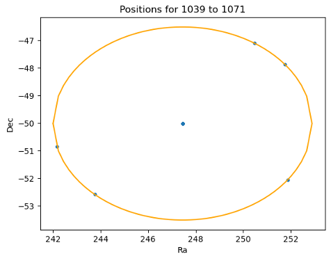
_images/snake.png — Fig. 1 Fig. 1: A sample set of points with the center position and 5 points offset by 3.5 degrees in a random direction. Credits Elana Urbach.#

The above circle illustrates the snake for a given target. The snake exercise was repeated for a grid of Az/Alt.

Data Description#

The data analyzed here was taking in three different nights, 9th, 17th, and 22nd March. The sequences number of each night were 600-1115, 292-858, and 569-1229,respectively. In total, we have 1592 exposures after discarding bad exposures.

The analysis was performed by joining all nights. Also, plots for each night were generated and the results were quite similar. The analysis for a individual night are also shown in the accompanion nootebook.

Residuals#

The residual for each slew is:

\[ \delta RA = Ra - <Ra> \]

The mean is taken over the three images acquired per slew. The same opperation was applied for DEC and the local coordinates Az/Alt.

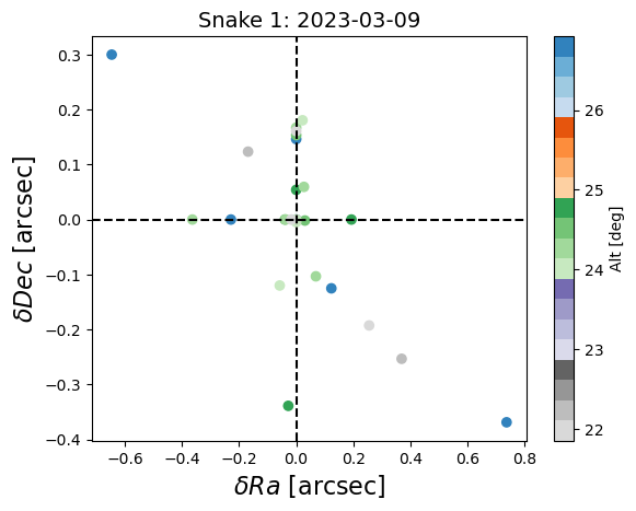
_images/residual_snake1.png — Fig. 2 Fig. 3: Residual sky coordinates for one snake exercise.#

To compute the sky precision we compute the standard deviation of the sky residuals.

Results#

The overall sky residual for 1016 exposures is presented below. Less than 0.5 percent of the data were outliers that we discarded.

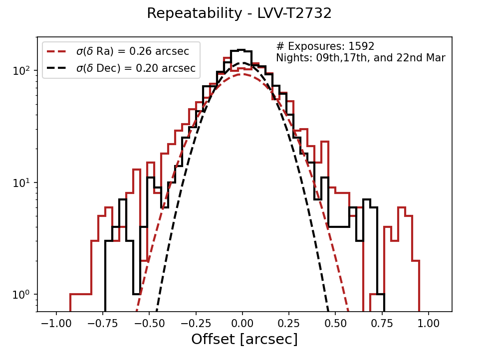
_images/radec_residual_histogram.png — Fig. 3 Fig. 3: Residual RADEC sky distribution of single targets#

The typical offset is \(\sigma(RA) = 26\) arcsec and \(\sigma(DEC) = 20\) arcsec.

Elevation And Azimuth Dependence#

For each snake I show the RA, DEC precision on a specified target.

There is no clear trend with elevation or azimuth. However, there are some points higher than specified requirement.

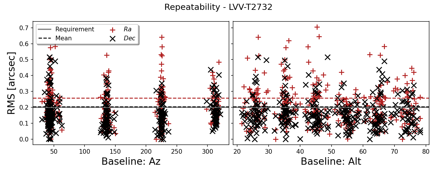
_images/scatter_radec_azalt.png — Fig. 4 Fig. 4: Sky precision RADEC as a function of elevation and azimuth.#

We note that RA precision is consitenly higher than Dec.

Pointing Model#

The pointing model introduces a drift on the exposures. The drift is a linear relation with time.

Below, we present the offset drift as a function of time offset since the baseline time. In this case, the baseline is the first exposure of the circle.

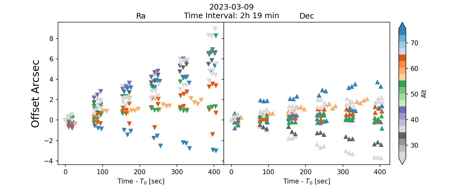
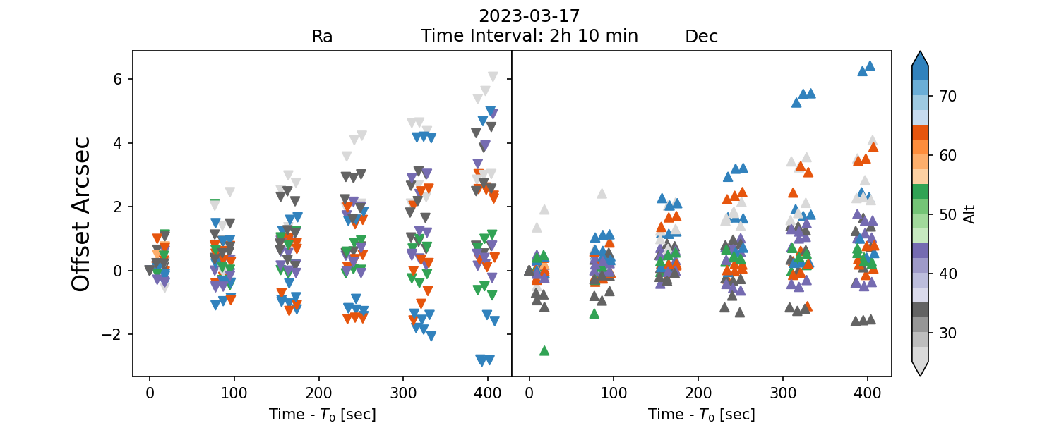
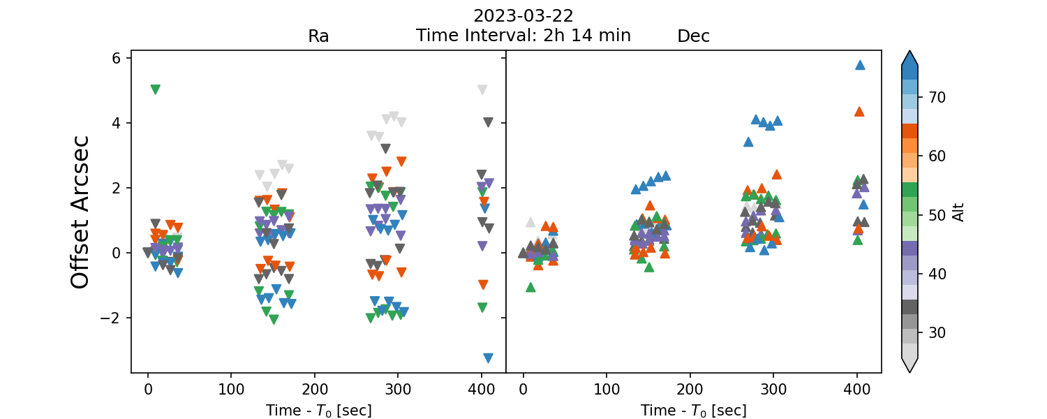
_images/offset_rate_2023-03-22.png — Fig. 5 Fig. 4: Drift offset as a function of elapsed time.#

The drift offset can be corrected by fiting a linear relation. In addition, the offset rate is basically the slope. However, for some cases we can see an anomolous behaviour. This outliers cases can be due to faults on the telescope components.

Assuming the linearity, below we show the offset rate distribution for each circle.

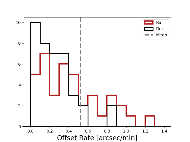
_images/offset_rate.png — Fig. 6 Fig. 5: Histogram of the offset rate.#

By correcting the drift offset, we can infer the actual TMA accuracy. The residual after correction shows RMS errors compared to the non drift analysis.

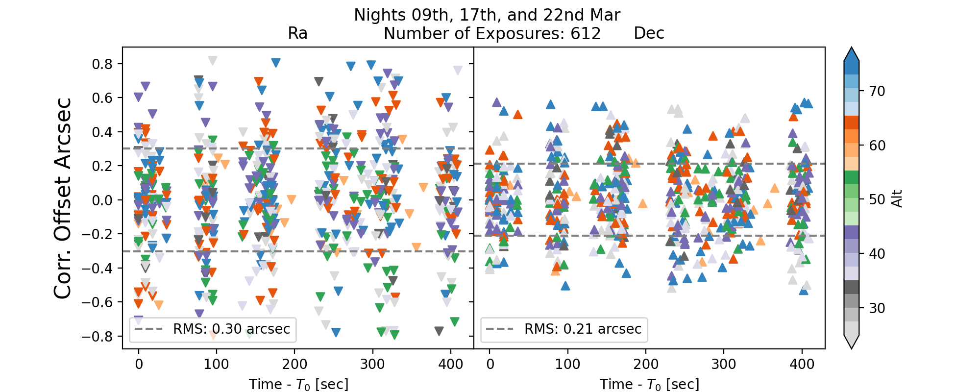
_images/corrected_offset_rate.png — Fig. 7 Fig. 6: Offsets residuals.#

The typical RMS is \(\sigma(RA) = 30\) arcsec and \(\sigma_{68}(DEC) = 21\) arcsec. Theses values are slighter higher, but not signficantly. The fitted linear model also introduces an intrinsic error.